Introduction

This report contains the basic and extended features that I implemented for the Nori2 path tracer, during the computer graphics course at ETH Zurich in 2020. Nori2 is an educational path tracer written in C++.

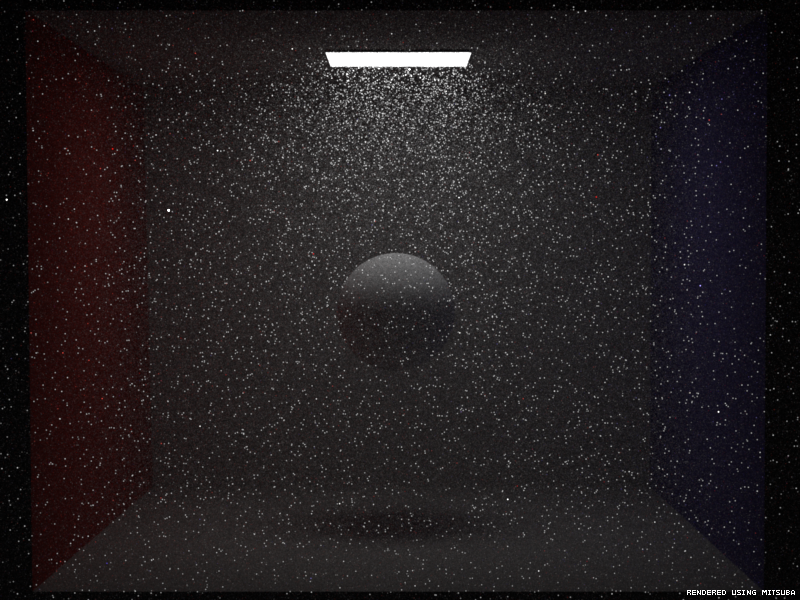
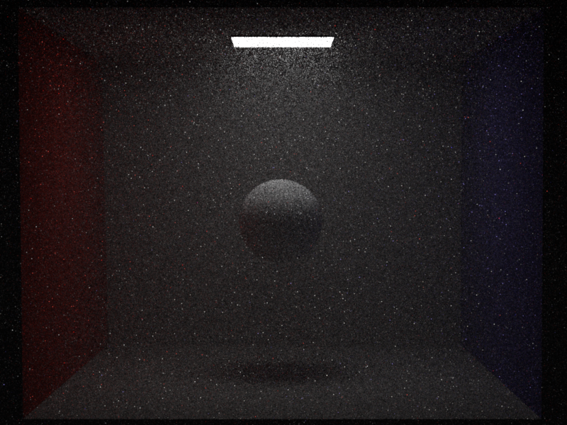
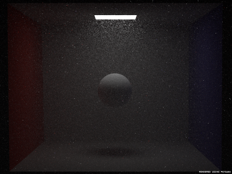
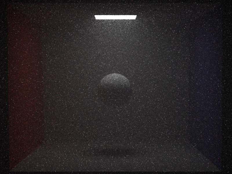
Average Visiblity Integrator

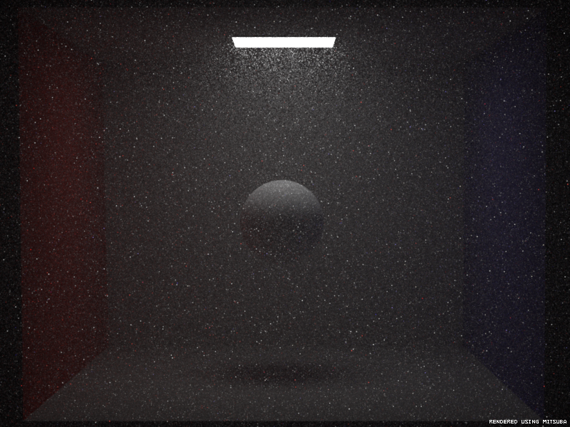
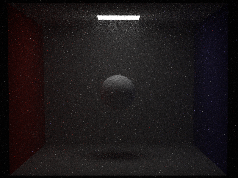
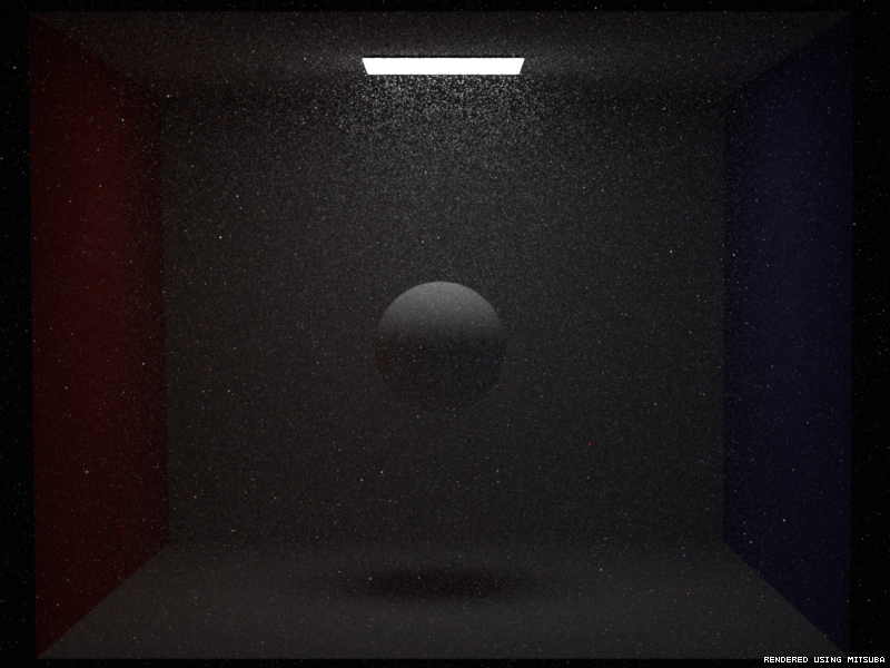
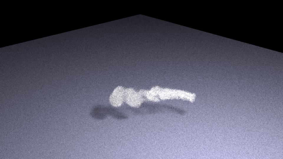
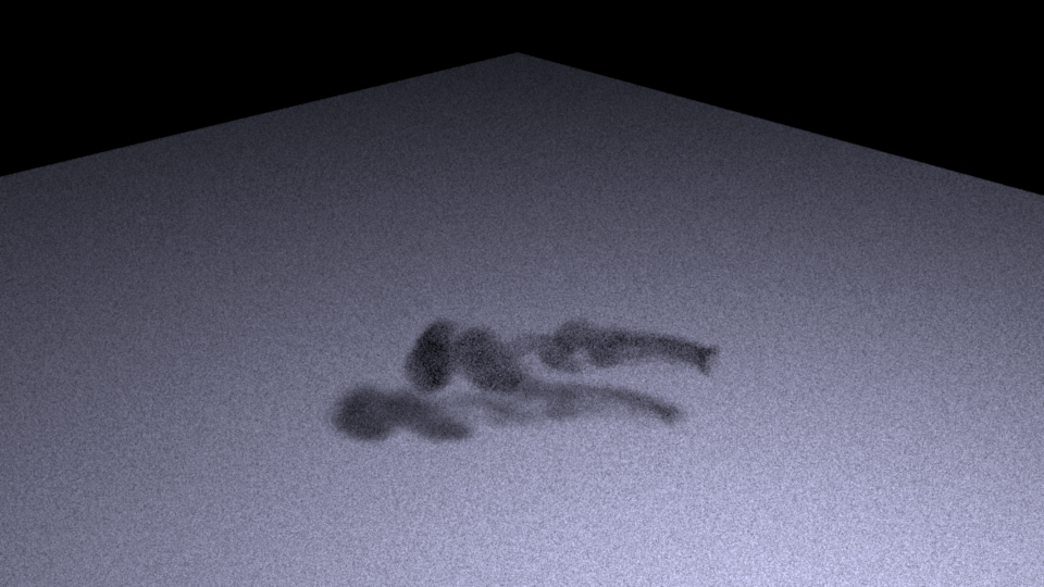
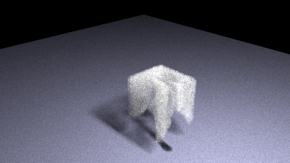
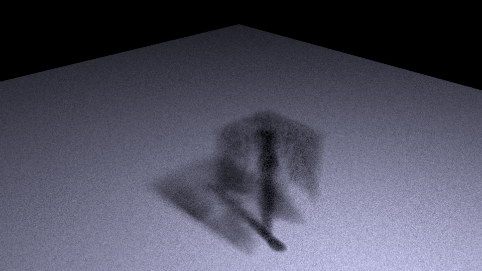
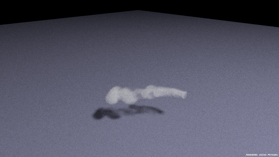
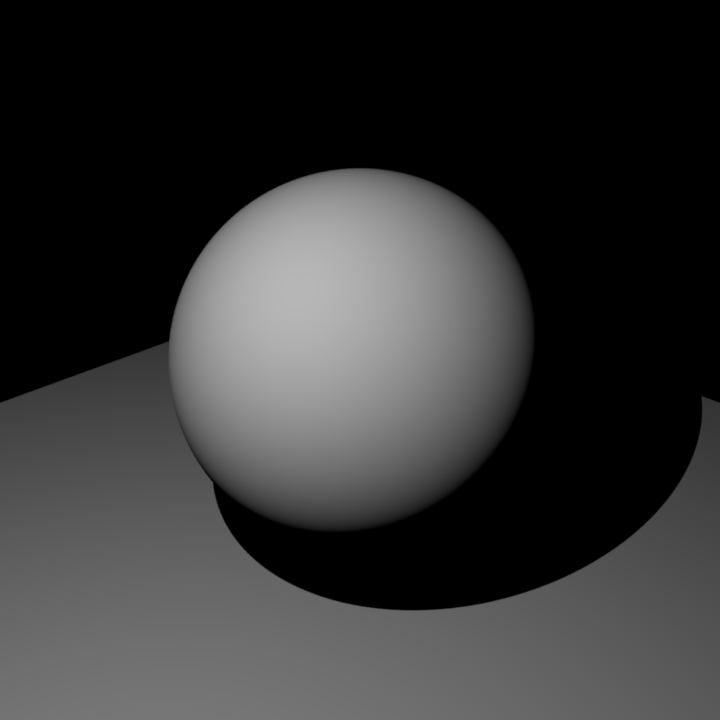
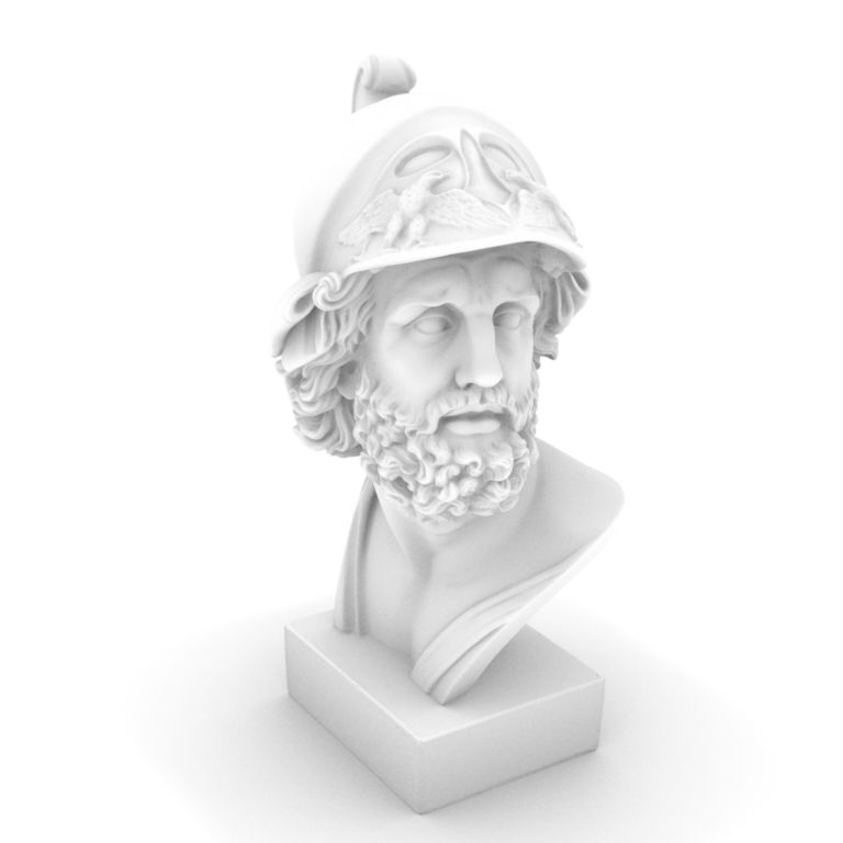
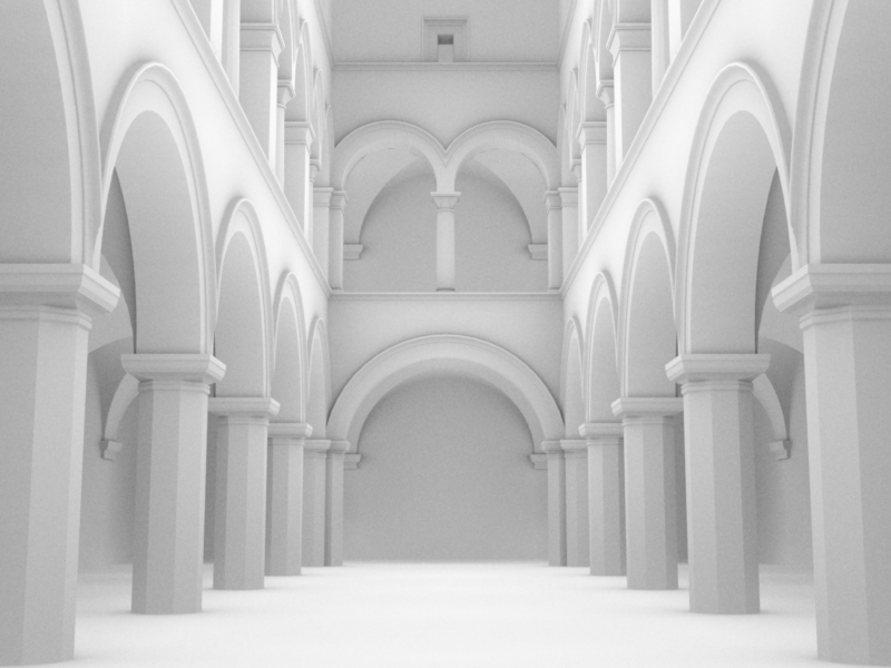
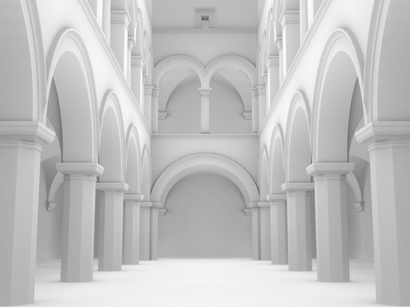
For each point intersected with the a camera ray, we sample random directions of its hemi-sphere (sampleUniformHemisphere) to construct a new ray in the corresponding direction. Under the ambient light case, if there is an intersection between the new ray and the mesh in the scene, the shaded color for this point should be black. This means that the ray is blocked and the pixel is black. Otherwise it should be shaded as the color of the ambient light. Finally, we average all the colors for each pixel's camera rays and return the average color. This task cost a some time when we use 1024 sample rays per pixel.

This feature is also known as ambient occlusion (AO), a method to approximate the global illumination in a scene. One interesting thing is that we can define min_t and max_t for the secondary constructed rays while detecting if the rays are blocked by other objects in the scene. Without doing this, the scene can be rendered as a black image when there is a closed box enclosing all the objects in the scene.

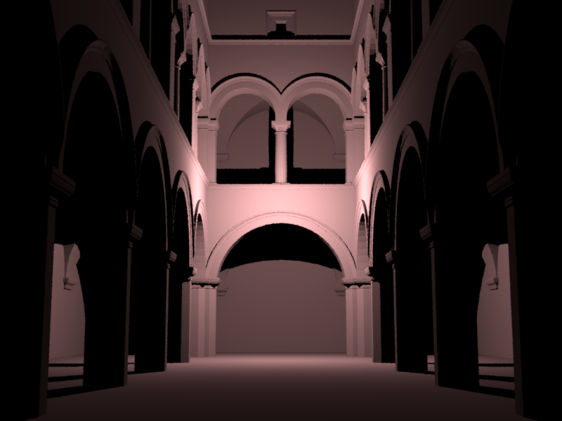
Rendered results of ajax and sponza are shown below.

AV Comparison: ajax

AV Comparison: sponza

Direct Illumination Integrator

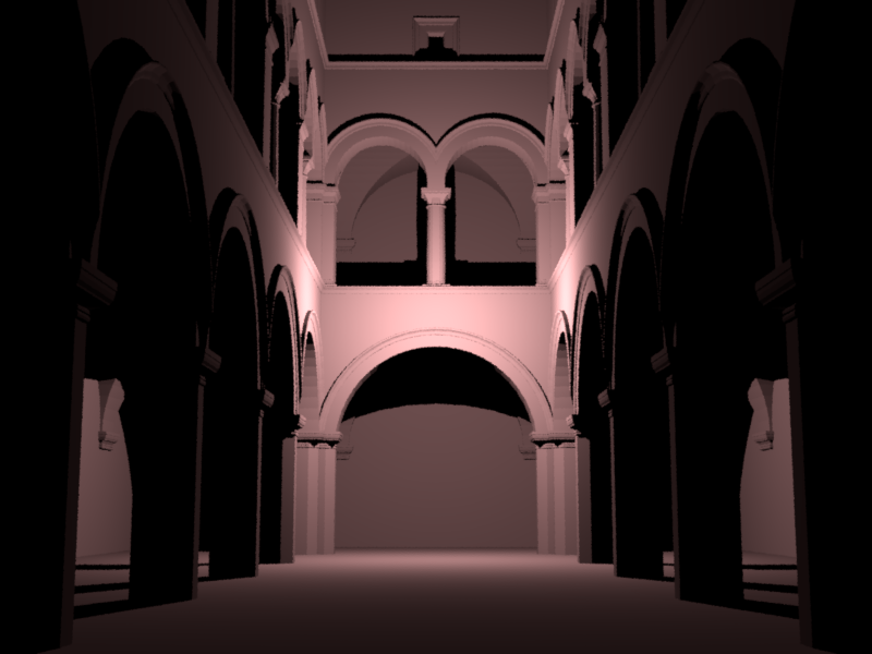
Here we consider implementing the point light class and its member functions. Different from other type of light sources such as area light, point light is considered as a infinitely small point without area. To render a shading point under a point light, the emmiter value is the pre-defined power of the point light divided by 4*PI and the distance from intersection to point light. The calculation of Li is similar to AO, the difference we need to consider is the BSDF value of the intersection point calculated in UV coordinate and the abs cosine angle between shading normal and the ray. More specficially, for each shading point, we sample one of the point light in the scene, as well as samplng BRDF outgoing direction for the intersection tests. The shading value is calculated by integration (sum here) of point light * BSDF * |cos_theta|.

Rendered direct illumination result of sponza is shown below.

DI Comparison: sponza

Light Sampling

In the following, we implement different sampling methods for rendering, including BRDF sampling, area light sampling and multiple importance sampling (MIS). First is light sampling.

Integrator Implementation

We note direct_ems as the integrator for sampling area light. For each primary camera ray, we sample a point on the light source, then construct the information in EmitterQueryRecord. Beides, for this primary intersection point, we also evaluate the BRDF value according to given information (wi, wo, etc.). Then we simply calculate all the terms needed in the rendering equation (also with cos(theta_o)).

Shape Area Light

There are 3 functions for implement a light source: eval() is for getting sampled value radiance, and pdf() for getting the sampled pdf. Notice that pdf should consider both solid angle conversion and distance from light source to shading point. This is based on change of variables in the integral equation. Then the sample function is to fill the EmitterQueryRecord and sample a secondary shadow ray given the primary camera ray. Lastly, the corresponding value is evaluated by eval/pdf.

Validation

Here are the results for sampling light source in the odyssey and veach scene:

odyssey_ems

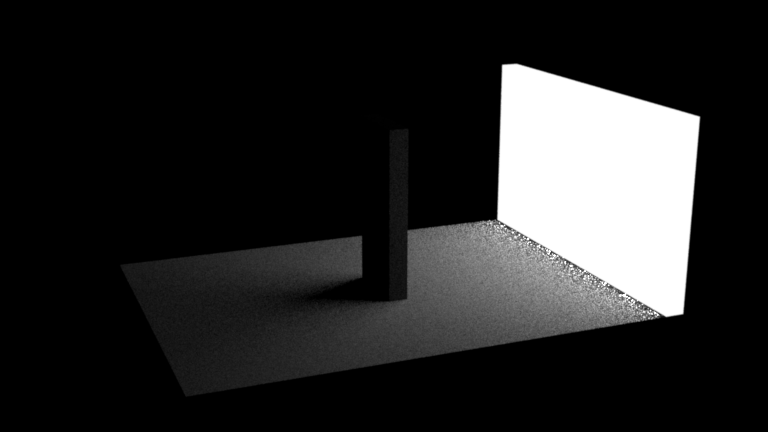
veach_ems

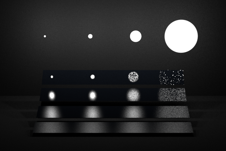
BRDF Sampling

BRDF sampling is another sampling technique. Instead of sampling a light source, we sample the bsdf's normal wh, direction wi and the corresponding values. (TODO: refactor details related to solid angle and microfacet BRDF)

Integrator Implementation

We note "direct_mats" as the BRDF sampling integrator, including sampling bsdf and evaluate the light radiance of the outgoing directions for each shading point. First we initialize a BsdfQueryRecord given wo (wi in nori), and then we sample bsdf normal then return the BRDF value. It will be multiplied by evaluated light radiance later.

Microfacet BRDF

Validation

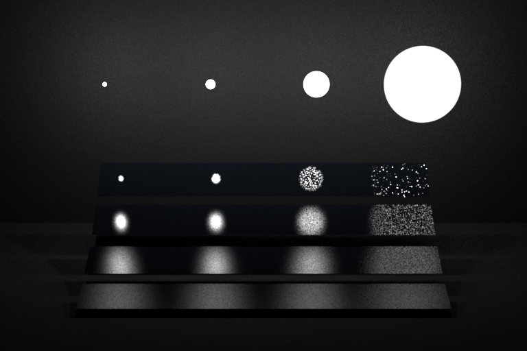
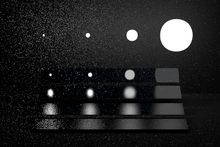
Here are the results of BRDF sampling for odyssey and veach scenees, with also warptests:

odyssey_mats

veach_mats

Part 3: Multiple Importance Sampling

MIS combines the advantages of both BRDF and light sampling.

Integrator Implementation

Here we combine the light sampling and the BRDF sampling implementation. (TODO: refactor details).

Validation

Here are the results from MIS for the odyssey and veach scenes, with screenshots of passed tests:

odyssey_mis

veach_mis

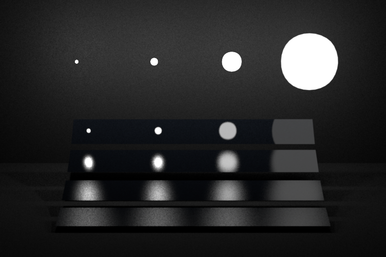
Image Validation

Two 4-way comparisons for each of the 2 scenes including direct_ems, direct_mats, direct_mis, together with the reference MIS rendering.

Path Tracing

path_mats Implementation

By adding a while loop and russianRoulette, we turn direct_mats into path_mats. We use russianRoulette with successProb = min(t, 0.99) .

path_mis

This is more trickly to implement. More details can be found in the code.

Validation

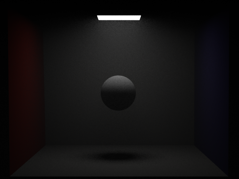
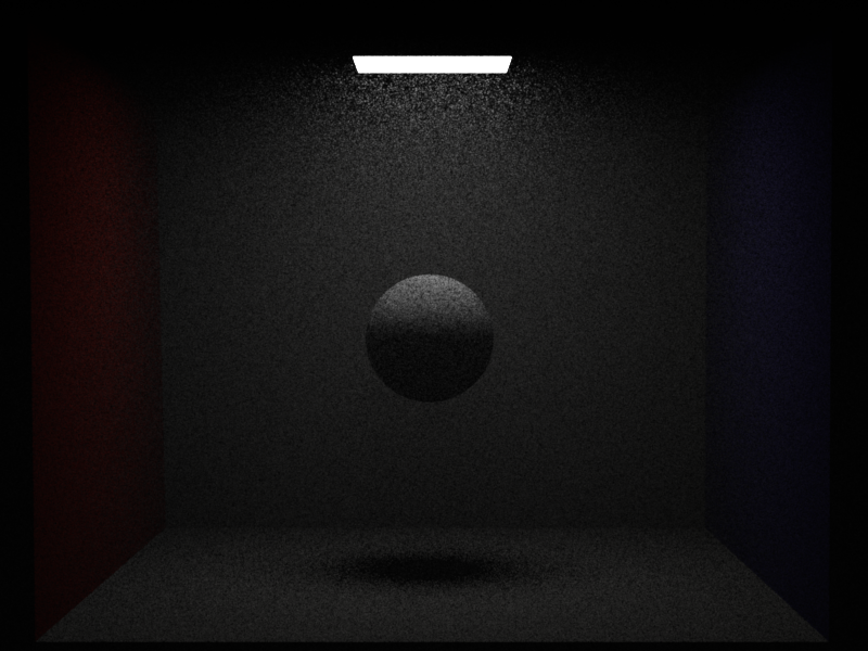
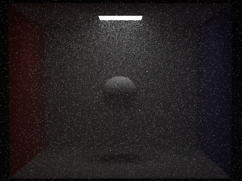
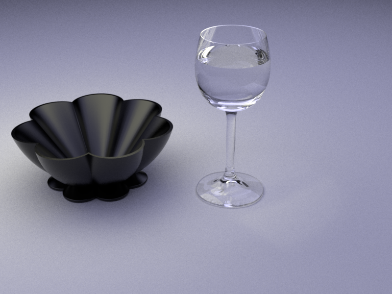
Here are two screenshots passing 2 tests. Then comes 3-way comparisons on 3 scenes:

Cornell box scene

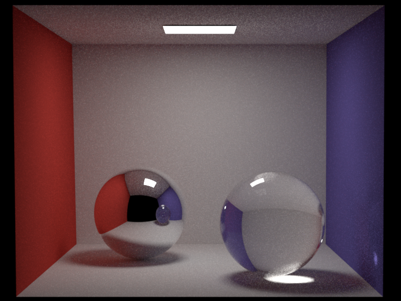
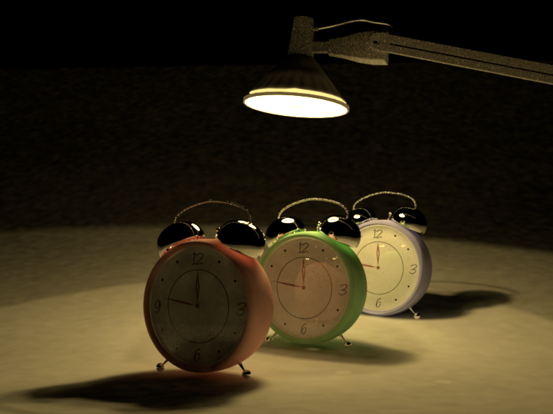
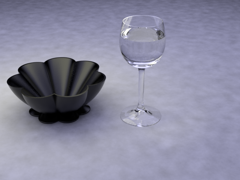
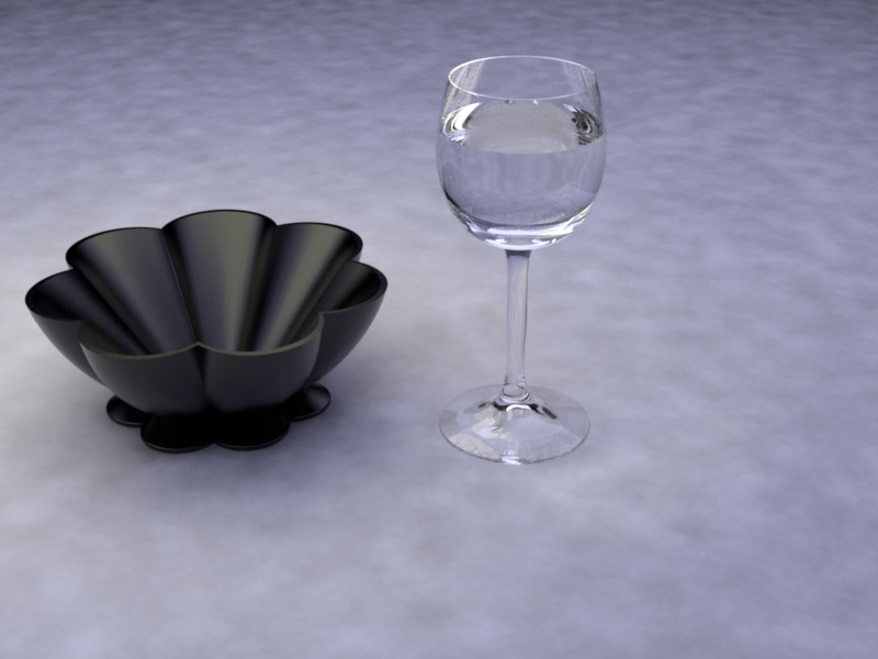
Table scene

Photon Mapping

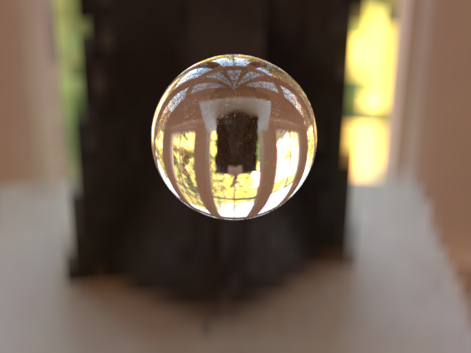
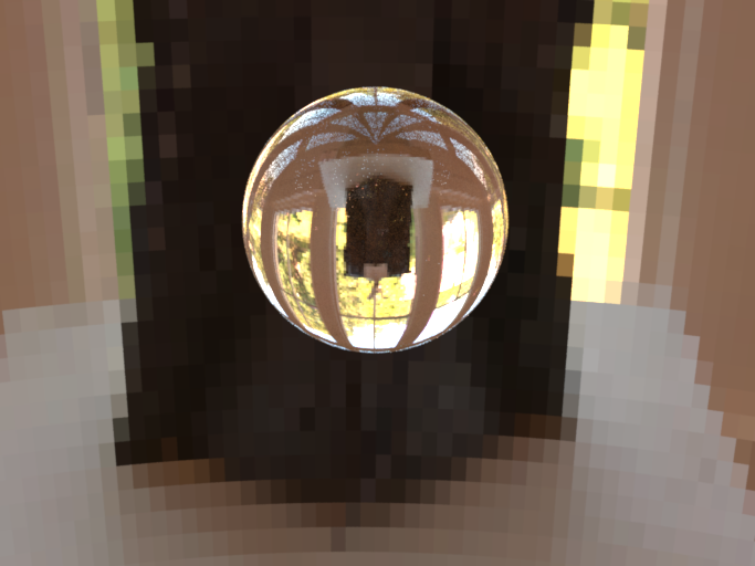
Overall, Photon Mapping is method good for rendering caustics, but usually slower than path tracing. This method is biased, and can introduce blocky artifacts when the number of photons is not large enough.

Implementation

Here we use two path tracing steps. Firstly, we emit photons from emitter in a while loop, and each photon will be stored for diffuse surface and sample new light ray until stopped by russianRoulette. After that, we do path tracing from the camera, and estimate the photon density on the diffuse surface. For delta BRDF, we simply use the same method as path_mats.

Validation

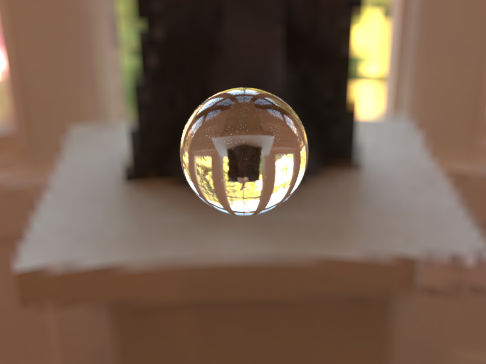
Here are three 2-way comparisons for all of the scenes: there are some differences on the backgroud because of randomness and minor difference between dielectric material.

Cornell box scene

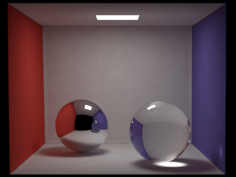
Table scene

Clocks scene

Equiangular Sampling in Single Scattering - 10 points

Implementation

We assume that we have already implemented the homogeneous medium and volumetric path tracer MIS. For single scattering, we terminate all light paths after the first bounce. Other are kept the same compared with volpath_mis distance sampling. Our goal is to replace the distance sampling by equiangular sampling. The idea is to consider the transmittance and its pdf in the first sampling step. Sampling equiangular distribution and its pdf is implemented in warp.cpp and we set the theta_b angle to be 90 degree. If the sampled distance is larger than tmax, then we get the pdf by 1 - cdf(tmax), which is done by an integration myself.

Validation

We compare single-scattering using distance sampling with equiangular sampling. It is shown that equiangular sampling brings an improvement in terms of noise reduction. The parameters in homogeneous are set to be: sigmaS = 0.2, 0.2, 0.2; sigmaA = 0.2, 0.2, 0.2; g of hg phase function is 0 and we use 32spp.

Heterogeneous Medium - 30 points

Homogeneous Medium with Volumetric Path Tracer MIS - 15 points

Implementation

In homogeneous case, we need to implement transmittance to attenuate light whenever we sample the emitter, and sampleFreePath by distance sampling. In homogenoues, we first check if our ray.o is inside the medium, if so then we start sampling distance and phase function to get the next ray.d. The transimittance of first path sampling is cancelled by its pdf. If distance < t_max during emitter sampling, we evalulate phase function (cosTheta between ray.d and lRec.shadowRay.d) just like bsdf and get w_ems. Then we sample phase function and evaluate emitter, get w_phase and update Li. Here we also use w_mat (not a new variable w_phase) to represent the weight of phase function sampling. Otherwise, if the sampled distance > t_max, we perform original emitter+BRDF MIS. Hitting surface also need to consider the transmittance while sampling emitter.

While sampling phase function(new direction), remember to change local direction to global based on ray.d.

Validation

Medium is filled in the whole scene in the following cases.

My volpath_simple (no phase MIS) VS. Mitsuba's volpath_simple: isotrophics phase, sigmaS = sigmaA = 0.2, 0.2, 0.2, 32spp:

My volpath_mis (emitter+bsdf, emitter+phase) MIS VS. Mitsuba's volpath: isotrophics phase, sigmaS = sigmaA = 0.2, 0.2, 0.2, 32spp:

Then we validation volpath_mis + hg phase function sampling (MIS) with Mitsuba, others paramters are the same. g = 0.7 and -0.7 in order for the folling two comparisons: Indeed, different g would change the performance of sample emitter (brighter or darker) compared with isotrophic.

Heterogeneous Medium with VolPath - 15 points

Implementation

In heterogeneous case, we use a bounding box and put varying density inside it. When we hit the bounding box we have two intersections paramterized by t_min and t_max. Then we delta tracking to sample a distance, again the first sample transimittance would be cancelled, which is a property of delta tracking in an un-biased way. The transmittance is also different from the one in the homogeneous case. Also, we use a constant albedo (1 or 0) for scattering and absorbtion, density would be tri-linearly interpolated. To implement this, we add a mediumInteraction following pbrt-v3 to manage the ray-medium interaction, when it's valid we sample by delta-trakcing, otherwise we do our original emitter+brdf MIS. Other parts would be the same in volpath_mis. The transmittance is also needed to be consider for surface-based emitter sampling inside the volume.

Validation

Here we use two data for validation. First one is downloaded from Mitsuba hetvol. We read the volume data source with python in ./smoke folder. Then we can easily read it into our heterogeneous.cpp class. Next one is a vdb data and we also preprocess it to numpy array and txt file to read it easily in nori. OpenVDB can be used to improve efficiency as a future work. We show the scattering and absorbing medium results in the following.

Mitsuba data: scattering with sigmaS = 5, 5, 5 and sigmaA = 0, 0, 0, g = -0.7 and rendered with 32spp, and vice versa:

VDB data: scattering with sigmaS = 5, 5, 5 and sigmaA = 0, 0, 0, g = -0.7 and rendered with 32spp, and vice versa:

I also try to compare the results with mitsuba using the same data, but my implementation needs a world to medium (toWorld) transformation matrix while Mistuab use the bounding box mesh. Then I found the mismatch between coordinate system of nori vs. mitsuba. We show a comparison with slightly different positions of camera, emitter and smoke (albedo = 1):

Images as Textures - 5 Points

Relevent Files:

1. src/imagetexture.cpp

First we need to load an image using the filesystem in nori. Then we find a way to map u, v values into the range [0, 1] using the reflect() function. Finally, remember to flip v value by v = 1 - v to get almost the same result compared with Mitsuba. Here we find that bilinear interpolation has marginal effect on the output.

Procedural Textures (perlin noise) - 5 Points

Relevent Files:

1. src/perlintexture.cpp

To implment perlin noise, we need to first define the width, height of the texture map, which are fixed to be 512 in the following example. Then we can use a 2D noise function to calculate the pixel values based on a hash table and use linear interpolation to smooth them.

There are two more parameters in perlin noise: depth and frequency. Here we can first see with higher frequency, we can see more dense texture in the followng figures with depth fixed to be 4:

In the following we can see with lower depth value, the color of texture becomes darker and sharper with frequency fixed to be 0.5:

Environment Map Emitter - 15 Points

Relevent Files:

1. src/envmap.cpp
2. scenes/project/emitter/nori-envmap.xml

Here comes a more advanced emitter: environment map emitter. To implement this, we first need to load an image like the "images as texture" feature. In the following figures, the setting between Nori and Mitsuba is still slightly different in terms of position or zoom-in.

But we are able to get similar results compared with mitsuba reference in terms of brightness, smoothness using the bilinear interpolation version. Without bilinear interpolation, we will suffer from blocked effect when the resolution of the image is low.